Understanding Einstein’s Relativity

The main idea

Einstein’s relativity gives a precise way to connect what different observers measure. In special relativity, observers moving uniformly relative to one another can disagree about elapsed coordinate time, distance, and which distant events happen together. Their measurements are related by exact equations, and they agree on physical coincidences, causal connections, and the elapsed time recorded by a particular clock along its particular journey. In general relativity, the geometry used for these measurements becomes a physical field related to matter and energy. Gravity is described through that geometry.

This guide builds those statements from simple experiments. You will derive time dilation, learn why simultaneity matters, calculate the age difference in a reunion experiment, and then see how gravity enters. The mathematics uses algebra, introductory calculus, and a small amount of linear algebra. The tensor equation at the end is a map of the next subject to learn, not a prerequisite for understanding the article.

Read Sections 1–8 for special relativity, Sections 9–13 for general relativity, and Section 14 for evidence and interpretation. Work the numerical examples on paper. The final questions, glossary, and equation reference are meant for a second pass. Throughout, an ideal clock means a physical clock whose ordinary disturbances have been controlled well enough that it measures the proper time along its path.

1 Start with an actual measurement

Imagine two observers passing each other in spacecraft. Each carries a ruler, a clock, and a lamp. What will they agree on? If one flashes the lamp, how fast does the pulse travel according to each observer? If their clocks separate and later meet, must they show the same elapsed time?

Newtonian mechanics begins with a common time: two frames can disagree about position and velocity while using the same elapsed time. If a train travels at speed $v$ and a passenger throws a ball forward at speed $u'$ relative to the train, the ground observer obtains $u=u'+v$. This is an excellent approximation at everyday speeds. Applying it to light would give $c+v$ for a forward pulse. Special relativity changes the rules connecting space and time so that every inertial observer measures the same vacuum light speed.

An event is something happening at a particular place and time, such as a flash reaching a detector. A frame labels it with coordinates $(t,x,y,z)$. The event is the physical occurrence; the four numbers are its address in that frame. Different addresses can identify the same event.

An inertial frame is a nonrotating frame in which a free test object moves at constant velocity. For the special-relativity examples here, neglect gravity. A frame is more than one person’s visual viewpoint: imagine a lattice of rulers and synchronized clocks spread throughout the region. A distant event receives the reading of the clock beside it. That construction separates a measured event time from the later moment at which its light reaches your eyes.

We use $c=299\,792\,458\ \mathrm{m/s}$, approximately $3.00\times10^8\ \mathrm{m/s}$. The symbol $\Delta$ means “final value minus initial value.” A prime, as in $t'$, labels a second frame; it does not mean a derivative.

2 The postulates and distant clock synchronization

Special relativity starts from two physical postulates:

1. The laws of physics have the same form in all inertial frames. No experiment confined to an isolated laboratory identifies an absolute uniform velocity.
2. Light in vacuum travels at speed $c$ in every inertial frame, independently of the motion of the source.

These statements do not require all observers to get identical numbers for every measurement. They require compatible laws and a consistent rule for translating the numbers. Einstein made the meaning of synchronized distant clocks central to that rule. [1]

Suppose clock A sends a light signal at its reading $t_1$. Clock B reflects it immediately. A receives it at $t_3$. In the standard Einstein synchronization convention, B’s reading at reflection is set to

This assigns equal outward and return travel times in that inertial frame. It gives an operational meaning to “at the same time” at different places. The directly measured round-trip time and this synchronization convention should be distinguished: defining the one-way travel times requires a convention for the distant clocks.

Example. A sends a pulse at 0 microseconds and receives it at 20 microseconds. B’s reflection is assigned time 10 microseconds. The distance is $c(10\ \mathrm{\mu s})\approx3.00\ \mathrm{km}$, where $1\ \mathrm{\mu s}=10^{-6}\ \mathrm{s}$.

Now consider two flashes simultaneous at opposite ends of a platform according to synchronized platform clocks. A moving observer can receive their signals at different times simply because the observer moves toward one signal. Reception times alone do not settle simultaneity. When the moving observer uses their own synchronized clock network and corrects for light travel, the two distant emissions are generally assigned different times. We will calculate the difference in Section 4.

3 Derive time dilation with a light clock

Build a clock from two parallel mirrors separated vertically by distance $L$. A light pulse goes from the lower mirror to the upper mirror and back. One round trip is one tick. Let $S'$ be the clock’s rest frame and $S$ an inertial laboratory in which the clock moves horizontally at constant speed $v$, with $0\leq v<c$.

The mirror separation is perpendicular to the motion. In the standard Lorentz transformation, transverse distances are unchanged; we derive that transformation’s longitudinal part in Section 4. The light-clock argument uses this transverse symmetry as well as the two postulates.

In $S'$, light travels total distance $2L$ at speed $c$. If the elapsed time on the clock itself is $\Delta\tau$, then

The Greek letter $\tau$ (“tau”) denotes proper time, the time recorded along the clock’s own path. In $S$, the mirrors move while light travels between them. Each half of the light path is diagonal. Let the laboratory’s round-trip coordinate time be $\Delta t$. During half that time, light travels distance $c\Delta t/2$ and the clock moves horizontally by $v\Delta t/2$.

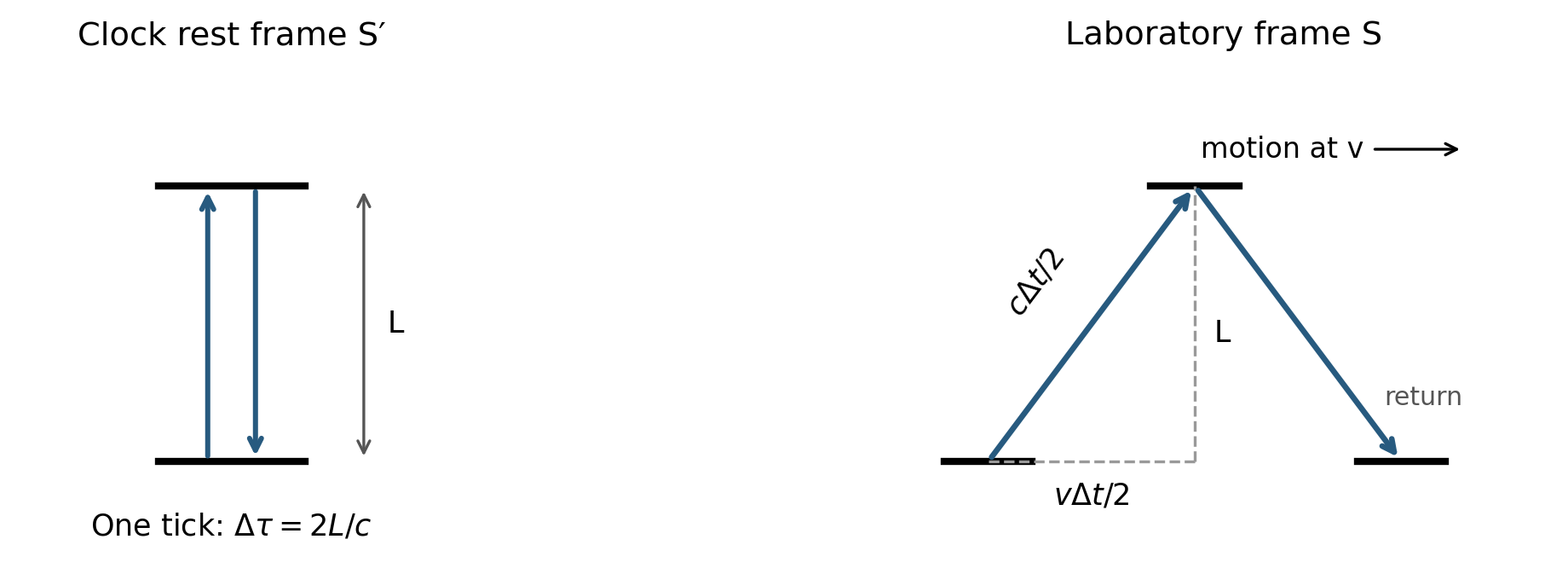
Pythagoras gives the relation between the hypotenuse and the two perpendicular sides:

Multiply every term by 4:

Subtract $v^2\Delta t^2$ and factor out $\Delta t^2$:

Divide by $c^2-v^2$, which is positive because $v<c$, then take the positive square root because elapsed time is positive:

Substitute $\Delta\tau=2L/c$ and define the Lorentz factor $\gamma$ (“gamma”):

For $v>0$, the denominator is less than 1, so $\gamma>1$. The laboratory assigns more time between the moving clock’s ticks. Equivalently, that clock accumulates $\Delta\tau=\Delta t/\gamma$ during a specified laboratory interval.

Example at $0.60c$. Calculate $v^2/c^2=0.36$, then $1-0.36=0.64$, then $\sqrt{0.64}=0.80$. Thus $\gamma=1/0.80=1.25$. During 10.0 laboratory seconds, the moving clock records $10.0/1.25=8.00$ seconds.

The observer beside the clock experiences ordinary local ticks. The comparison is between measurements made along different paths or using different clock networks. Also, time dilation is not simply what a telescope shows: incoming pulse intervals additionally depend on the changing source-to-observer distance, the Doppler effect.

Why should an atomic clock follow a light-clock result? If two otherwise reliable clocks at rest together disagreed merely because their common uniform velocity changed relative to another frame, a laboratory could use that disagreement to identify preferred motion. Relativity instead predicts a universal relation for ideal clocks. Actual clocks can also respond to temperature, fields, or mechanical stress; those effects require separate control. Experiments test whether different physical processes follow the predicted relation. [5, 6]

4 Space and time must transform together

Let $S'$ move at constant velocity $+v$ along the $x$ axis of $S$. Choose parallel axes and coincident origins at $t=t'=0$. The standard Lorentz transformation is

Here is a derivation of the two coupled formulas. Uniform space and time lead us to seek a linear transformation. The moving origin satisfies $x=vt$ and must have $x'=0$, so write $x'=A(x-vt)$. Write the time transformation as $t'=Bt+Dx$, with coefficients depending on $v$.

For a right-moving light pulse, $x=ct$ and $x'=ct'$. Substituting and dividing by $t$ gives

For a left-moving pulse, $x=-ct$ and $x'=-ct'$. Substituting gives

Subtract the second equation from the first: $2Ac=2cB$, so $B=A$. Add the equations: $-2Av=2c^2D$, so $D=-Av/c^2$. Therefore $t'=A(t-vx/c^2)$.

The relativity principle and spatial isotropy imply that the inverse transformation has the same scale factor with velocity reversed: $x=A(x'+vt')$. Substitute the formulas already obtained:

The $-vt$ and $+vt$ terms cancel, leaving

For arbitrary $x$, the coefficient must be 1. Thus $A^2=1/(1-v^2/c^2)$. Choose the positive root to preserve the direction of time and approach the identity at $v=0$: $A=\gamma$. This is the Lorentz transformation under the stated symmetry and synchronization assumptions. [1, 2]

The crucial new term is $-vx/c^2$: assigning time in another frame requires knowing position. For two events, subtract their transformed times:

If they are simultaneous in $S$, then $\Delta t=0$. Consequently,

Example. Let event B occur 300 m to the right of event A, with both occurring at the same $S$ time. Take $v=0.60c$ and $\gamma=1.25$. Using $c\approx3.00\times10^8\ \mathrm{m/s}$,

Thus B is assigned a time 0.750 microseconds earlier than A in $S'$. Both frames agree on what each event is. They use different slices of distant spacetime as “now.” Events at the same place and time cannot be separated by a change of frame; physical coincidences remain coincidences.

5 Proper time is what a clock accumulates

For neighboring events on a clock’s path in flat spacetime, the invariant interval is

“Invariant” means every inertial frame obtains the same value for this combination. Individual coordinates change. You can verify invariance by substituting the Lorentz transformation; the mixed space-time terms cancel. The minus signs are essential: spacetime geometry differs from ordinary Euclidean distance.

Define the clock’s coordinate speed by $v^2=(dx/dt)^2+(dy/dt)^2+(dz/dt)^2$. Divide the interval equation by $c^2dt^2$:

Taking the positive root yields $d\tau=dt\sqrt{1-v^2/c^2}$. If the speed changes, add the contributions along the entire path using an integral:

Here $t_A$ and $t_B$ are the departure and arrival coordinate times; $\tau$ denotes elapsed proper time between them. This formula works for accelerated paths in flat spacetime, provided the clock behaves ideally. Special relativity can describe acceleration. It does not require all objects to move uniformly; inertial coordinates are the convenient background for the calculation.

An interval between two events and the proper time along a path connecting them are distinct. For an inertial straight path, the endpoint interval directly gives its proper time. For an accelerated path, integrate along that path. Different paths between the same events can accumulate different proper times.

For causal structure, an event separation is timelike when $c^2\Delta t^2>\Delta x^2+\Delta y^2+\Delta z^2$, null when the quantities are equal, and spacelike when the inequality is reversed. Massive objects follow timelike paths; vacuum light follows null paths. No ordinary signal traveling at or below $c$ connects spacelike-separated events. Their order may differ between frames without reversing cause and effect. A light ray has zero proper time along its path, but there is no valid inertial “rest frame of a photon.”

6 Length contraction and adding velocities

Measuring a moving length

A rod’s proper length $L_0$ is its length in its rest frame. Suppose it lies along $x'$ and moves at speed $v$ relative to $S$. To measure its length in $S$, record both endpoint positions at the same $S$ time. This condition is $\Delta t=0$.

Subtract the transformed endpoint positions:

The endpoints remain at fixed positions in the rod frame, so their position difference is $\Delta x'=L_0$, even though the selected endpoint events are not simultaneous there. Set $\Delta x=L$ and $\Delta t=0$:

A 100 m rod moving lengthwise at $0.60c$ has measured length $100/1.25=80.0$ m in $S$. It remains 100 m in its rest frame. This result is about simultaneous endpoint measurements in specified frames; a photograph also contains light-travel-time effects. No comparable contraction occurs perpendicular to the relative motion.

Deriving the velocity rule

For motion along the shared axis, let $u=dx/dt$ and $u'=dx'/dt'$. Since $v$ and $\gamma$ are constant, differentiate the Lorentz formulas:

Divide the first differential by the second, cancel $\gamma$, and divide numerator and denominator by $dt$:

To solve for $u$, multiply through and collect its terms:

If a spacecraft moves at $0.60c$ and launches a probe forward at $0.60c$ in its own frame, the original frame measures

For a forward light pulse, substitute $u'=c$. The numerator becomes $c+v=c(1+v/c)$; the denominator is $1+v/c$. Their ratio is exactly $c$. At speeds much smaller than $c$, the product $u'v/c^2$ is tiny and the Newtonian rule is recovered.

7 A complete reunion calculation

Two ideal clocks start together at event A. Clock E remains at $x=0$ in an inertial Earth-like frame. Clock T travels to a station 4.00 light-years away at $0.80c$, reverses direction, and returns at the same speed. Ignore gravity and approximate the turnaround as brief enough to contribute negligible duration. A light-year is a distance: the distance light travels in one year.

The outbound coordinate time is distance divided by speed:

The inbound leg also takes 5.00 years, so E records 10.0 years. For T,

Each leg contributes $5.00/(5/3)=3.00$ proper years. T records $3.00+3.00=6.00$ years. At reunion the clocks are beside each other: the difference is 4.00 years, independent of distant synchronization conventions.

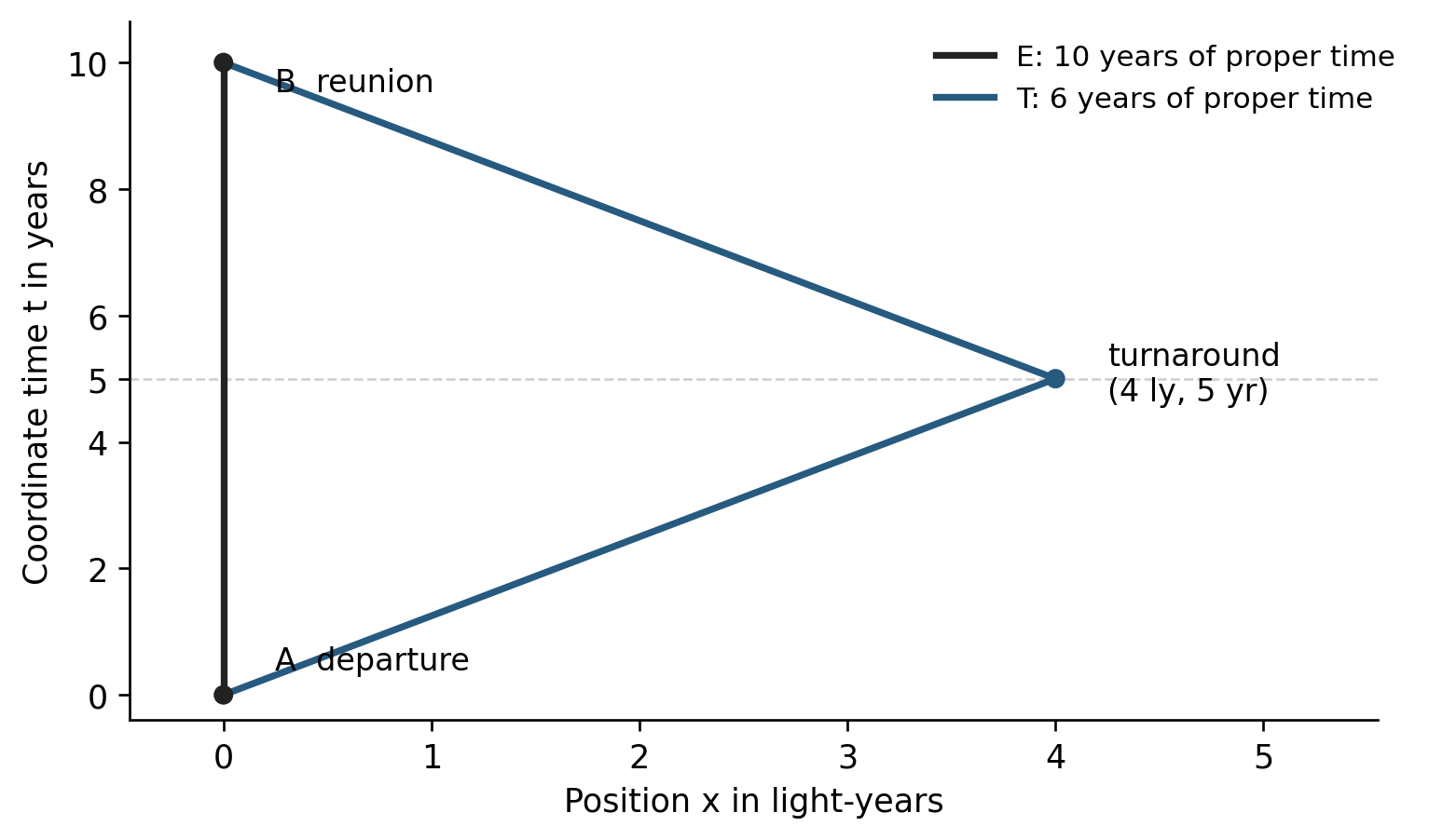
Why cannot T make an identical argument that E must age less? During each cruising leg, T uses a different inertial frame. At turnaround, the set of distant Earth events assigned “simultaneous with me now” changes. E uses one inertial frame throughout the idealized trip. The two complete paths are physically different. [4]

We can quantify that change without claiming that Earth’s clock jumps. In units with $c=1\ \mathrm{ly/yr}$, the outbound Lorentz time at turnaround is $(5/3)(5-0.8\times4)=3$ years. At Earth, $x=0$, so the event with that outbound-frame time has $(5/3)t_E=3$, giving $t_E=1.8$ years. For the inbound comoving frame, simultaneity with turnaround requires

Thus the inbound assignment is $t_E=8.20$ years. The assignment changes by 6.40 years in the instantaneous-turnaround idealization. During each 3.00-year cruise, T assigns Earth $3.00/(5/3)=1.80$ years of aging. The complete accounting is $1.80+6.40+1.80=10.0$ years. No physical clock abruptly advances by 6.40 years; the traveler changes how distant events are grouped into a simultaneous slice. A finite turnaround makes this reassignment continuous.

Acceleration enables the change of path and frame, but there is no universal rule that acceleration itself subtracts a fixed amount of aging. The accumulated result comes from integrating proper time. Ordinary acceleration-induced disturbances of a real clock are additional instrumental effects.

8 Energy and momentum belong to the same structure

Relativistic mechanics must make energy and momentum conservation compatible with Lorentz transformations. For a massive particle of invariant mass $m>0$, the resulting expressions are

Here $E$ is total energy, $\mathbf{p}$ is momentum, and the bold symbols are three-dimensional vectors. These formulas introduce relativistic dynamics; the light-clock triangle alone does not derive them. The four components $(E/c,p_x,p_y,p_z)$ form a four-vector whose invariant norm gives a useful identity.

Write $p^2=p_x^2+p_y^2+p_z^2=\gamma^2m^2v^2$. Then subtract explicitly:

Factor out $\gamma^2m^2c^4$:

The last equality uses $\gamma^2(1-v^2/c^2)=1$. Therefore

At rest, $p=0$, so the positive energy is $E_0=mc^2$. This is rest energy. Kinetic energy is the excess over rest energy:

When $v\ll c$, the binomial expansion gives $(1-v^2/c^2)^{-1/2}\approx1+v^2/(2c^2)$. Substitute it into $K$: the 1 terms cancel, leaving $K\approx[v^2/(2c^2)]mc^2=mv^2/2$. Newtonian kinetic energy is the low-speed limit.

Example. For $m=1.00\ \mathrm{kg}$ and $v=0.60c$, $E_0\approx9.00\times10^{16}\ \mathrm{J}$, $E=1.25E_0\approx1.13\times10^{17}\ \mathrm{J}$, and $K=0.25E_0\approx2.25\times10^{16}\ \mathrm{J}$. The rest-energy value does not mean an ordinary kilogram is an available energy source that can simply be emptied.

We keep $m$ invariant instead of describing mass as increasing with speed. For a massive object, reaching $c$ would require $\gamma$ and its energy to diverge. A photon has $m=0$ and obeys $E=pc$; it has no rest frame. For a composite system, rest mass includes internal kinetic and binding energy through the system’s total rest-frame energy. Energy leaving a system can reduce its mass. [2]

9 Why gravity requires another step

Special relativity describes physics on flat spacetime. General relativity makes spacetime geometry dynamical and uses it to describe gravity. Its starting clue is the common free fall of bodies with different composition, when air resistance and other forces are negligible.

Imagine a small sealed elevator freely falling near Earth. Release a pen beside you. For a short interval it floats beside you because you and the pen share nearly the same free-fall motion. A small freely falling laboratory therefore approximates an inertial special-relativistic laboratory. Conversely, an accelerating rocket in otherwise empty flat spacetime makes released objects accelerate toward its floor relative to the cabin. The floor pushes on standing occupants.

The Einstein equivalence principle says that local nongravitational experiments in a sufficiently small freely falling laboratory follow the laws of special relativity. “Local” matters: a large laboratory can detect differences in free-fall acceleration across its extent. Two falling objects separated sideways near Earth tend toward Earth’s center along slightly converging directions; two separated vertically experience different accelerations. These are tidal effects. [3]

Standing on the ground is therefore different from free fall. The ground supplies an upward contact force. An accelerometer at rest on the ground reads a nonzero proper acceleration, while an ideal freely falling accelerometer reads zero. Coordinate acceleration and accelerometer-measured acceleration are different quantities.

The equivalence principle guides the theory, but by itself it does not uniquely produce the complete Einstein field equations. Those equations add a specific dynamical relationship between spacetime geometry and the distribution of energy, momentum, and stress.

10 Curved paths and curved spacetime are different

A worldline is an object’s path through spacetime. A rocket firing its engines can have a curved worldline even when spacetime is flat. Likewise, curved coordinate-grid lines on a flat sheet do not bend the sheet itself. Neither a curved plotted trajectory nor position-dependent coordinate formulas automatically establish intrinsic curvature.

Spacetime curvature concerns relations among neighboring paths and measurements over a region. Freely falling, initially neighboring objects can develop relative acceleration even when neither experiences a nongravitational force. The mathematical object called the Riemann curvature tensor describes such tidal structure. Choosing clever coordinates can remove certain apparent gravitational terms at a point, but cannot remove nonzero curvature even at that event.

A geodesic is a path that is locally straight according to the spacetime geometry. An ideal freely falling massive test particle follows a timelike geodesic; a light ray in vacuum follows a null geodesic in the geometric-optics approximation. In a suitable small freely falling frame, either path looks locally straight. Across a larger curved region, those local frames fit together differently from frames in flat spacetime.

For a massive free particle, the proper-time version of the geodesic principle says the path makes proper time stationary under small path variations with fixed endpoints. For sufficiently short segments it locally maximizes proper time. The stronger claim that every geodesic is the globally longest-time path between arbitrary distant events would be false.

An orbit can consequently curve in its spatial projection while being a free-fall spacetime geodesic. “Straightest through spacetime” and “straight line across a spatial map” answer different questions. The familiar rubber-sheet picture has limited value: it depicts only a spatial surface, uses external gravity to pull objects down, and omits the time part of spacetime. It is not the mechanism of general relativity. [3]

11 Gravitational clock differences

For a stationary, nonrotating spherical source of mass $M$, the exterior Schwarzschild geometry gives the rate of a clock held at a fixed spatial position, with constant radius $r$ and constant angular coordinates:

Here $G$ is Newton’s gravitational constant, $r$ is the areal radius (a sphere at that radius has area $4\pi r^2$), and $t$ is Schwarzschild coordinate time normalized to a stationary clock far away. The formula applies outside the source and outside $r=2GM/c^2$. This stationary clock is being supported rather than freely falling; an orbiting clock needs a formula that includes its motion. Rotation and nonspherical structure require a more complete model.

For two such clocks at radii $r_A$ and $r_B$, divide their accumulated proper times over the same coordinate interval:

If B is higher, $r_B>r_A$, then $2GM/(r_Bc^2)$ is smaller. The numerator is larger, and the ratio exceeds 1. The higher stationary clock accumulates more proper time per common coordinate interval. This is a comparison between clocks, while every observer still measures normal local seconds.

Near Earth’s surface, for small height differences and a weak gravitational field, use Newtonian potential $\Phi=-GM/r$. Since $|\Phi|/c^2\ll1$, expand the square root using $\sqrt{1+\epsilon}\approx1+\epsilon/2$:

To first order, the ratio between two clock rates is $1+(\Phi_B-\Phi_A)/c^2$. Over a small height increase $h$, $\Phi_B-\Phi_A\approx gh$, where $g$ is the local gravitational acceleration. Let $f_A$ and $f_B$ denote ticks per unit of the same coordinate time, or the equivalent signal-corrected clock comparison. Identical clocks still have the same ticking frequency when each is measured against its own local proper time. With $\Delta f=f_B-f_A$ and $f=f_A$, the higher-minus-lower fractional rate difference is

Example at 100 m. With $g=9.81\ \mathrm{m/s^2}$ and $c\approx3.00\times10^8\ \mathrm{m/s}$, compute $gh=981\ \mathrm{m^2/s^2}$ and $c^2=9.00\times10^{16}\ \mathrm{m^2/s^2}$. The units cancel, giving $\Delta f/f\approx1.09\times10^{-14}$. Multiply by $86\,400\ \mathrm{s}$ per day:

The higher clock gains about 0.942 nanoseconds per day relative to the lower one in this approximation. Here $1\ \mathrm{ns}=10^{-9}\ \mathrm{s}$.

Motion and gravitational environment can both contribute. In suitable weak-field coordinates, for speeds much smaller than $c$,

Higher potential contributes a positive change; higher coordinate speed contributes a negative change. This formula neglects higher-order and rotational effects. It is useful for understanding why an orbiting clock comparison needs both terms; it is not a universal formula for arbitrary strong fields.

Gravitational redshift is closely related: a light signal emitted lower down and received by a higher stationary observer has a lower measured frequency than an identical local standard at reception. For the same Schwarzschild setup, the locally measured received-to-emitted frequency ratio is the inverse of the stationary clock-rate ratio:

The faster upper clock counts fewer arriving wave cycles per local second. Here the frequencies are measured locally at emission and reception, unlike the common-coordinate-time ticking rates above. Importantly, stationary clocks in an accelerating coordinate system in flat spacetime can also have position-dependent rates. A redshift measurement alone is therefore not a unique proof of nonzero spacetime curvature. Tidal measurements and the broader gravitational predictions supply additional information.

12 The mathematics behind the geometry

Your linear algebra provides a useful starting point. In Euclidean space, a small displacement has squared length $dx^2+dy^2+dz^2$. In special relativity, the corresponding spacetime expression is $c^2dt^2-dx^2-dy^2-dz^2$. General relativity replaces those fixed coefficients with a position-dependent metric, $g_{\mu\nu}$. Along a timelike clock path, its proper time satisfies

We use the $+---$ sign convention and $x^0=ct$, $x^1=x$, $x^2=y$, $x^3=z$. The superscripts here label coordinates; they are not powers. The indices $\mu$ and $\nu$ each run from 0 to 3. The displayed double sum means multiply each metric entry by the corresponding pair of coordinate displacements and add all 16 terms. Because the metric is symmetric, it has 10 independent entries.

In matrix language this is a quadratic form, $d\mathbf{X}^{\mathsf T}g\,d\mathbf{X}$, where $d\mathbf{X}$ is a column of four coordinate displacements and $\mathsf T$ denotes transpose. In a local inertial frame the metric takes the diagonal form $(1,-1,-1,-1)$ at the event. In general coordinates it can contain mixed terms such as $dt\,dx$.

Position-dependent metric entries do not by themselves imply curvature: even flat space has position-dependent coefficients in polar coordinates. Curvature is calculated from particular combinations of the metric and its derivatives. This is where multivariable calculus develops into differential geometry.

The Einstein field equation is usually written

The symbols name different physical and mathematical objects:

• $G_{\mu\nu}$ is the Einstein tensor, built from curvature. It is not the same object as the constant $G$ without indices.
• $\Lambda$ is the cosmological constant. It contributes a term proportional to the metric.
• $T_{\mu\nu}$ is the stress-energy tensor, encoding energy density, momentum density and flux, and stresses including pressure.
• $8\pi G/c^4$ sets the coupling strength between those quantities in the chosen units.

More explicitly, $G_{\mu\nu}=R_{\mu\nu}-\tfrac12R g_{\mu\nu}$, where $R_{\mu\nu}$ is Ricci curvature and $R$ is its scalar contraction. You do not need to calculate these objects to understand the equation’s role: given matter, boundary or initial data, and appropriate physical conditions, solve for a metric consistent with them. Then use that metric to predict clock readings, light propagation, and free-fall motion. [7]

The equation is a coupled nonlinear set of differential equations. A useful subtlety is that an empty region with $T_{\mu\nu}=0$ need not have zero curvature. The region outside a star can have tidal curvature; gravitational waves can also pass through vacuum. Matter at each point does not determine every curvature component there by a simple local proportionality.

13 Light and the meaning of time bending

In curved spacetime, every observer still measures vacuum light speed $c$ locally, including an accelerated observer. Over an extended region, light follows the spacetime geometry, producing gravitational lensing and propagation-time delays. A coordinate speed such as $dr/dt$ can vary with the coordinate system. That variation alone is not a local measurement of light slowing below $c$.

For weak deflection outside an approximately spherical, nonrotating mass, general relativity predicts total light deflection

where $\alpha$ is in radians and $b$ is the impact parameter, approximately the closest approach distance in the weak-deflection limit. This is a stated result of solving the null-geodesic problem, not a derivation supplied here. Its assumptions matter; rays near a black hole require a stronger-field treatment.

The phrase time bending can hide several different ideas. For learning, replace it with the measurable or mathematical statement intended:

1. Relative motion can give different clock readings, even in flat spacetime.
2. Clocks held at different gravitational potentials can have different rates relative to a common stationary comparison.
3. Intrinsic spacetime curvature produces tidal structure and affects the relation among neighboring free-fall and light paths.

These are connected within relativity, but they are not synonyms. Time dilation does not automatically mean curvature; a bent worldline does not automatically mean curved spacetime. Nothing in the calculation requires imagining time as a material ribbon folding into another dimension.

14 Evidence and the limits of the claim

Thought experiments establish consequences of assumptions. Measurements determine whether nature follows them. Three complementary examples illustrate the difference:

Optical clock comparisons. Chou and colleagues compared aluminum-ion clocks and resolved relativistic effects from controlled motion and from raising one clock by 33 cm. That height change produced a measured fractional frequency change of $(4.1\pm1.6)\times10^{-17}$. The moving-ion experiment was a separate part of the study. These are measured frequency comparisons, with other systematic shifts controlled. [5]

Fast ion spectroscopy. Botermann and colleagues used lithium ions moving at $0.338c$ and opposing lasers to test a relativistic Doppler/time-dilation relation. Their reported dimensionless deviation from the special-relativistic prediction was $(1.5\pm2.3)\times10^{-9}$, consistent with zero. The uncertainty concerns that particular measured combination and test model, not every possible alternative to relativity. [6]

Gravitational waves. The LIGO and Virgo collaborations reported the signal GW150914, observed in 2015, whose changing waveform agreed with general-relativistic predictions for a binary black hole merger and the resulting remnant. This tests dynamical gravity through a different observable from a clock-rate comparison. [8]

These examples are part of a much larger body of tests. A theory earns support by explaining multiple observables with one consistent structure. No finite collection of experiments proves that every equation will hold in every untested regime.

There is also a difference between measurable physics and metaphysical language. All clocks are physical processes. Saying that a clock’s internal processes differ in rate relative to another clock can correctly describe an observation. Relativity adds the quantitative rule, specifies which comparisons are meaningful, and connects clocks to lengths, momentum, light propagation, and gravity. An interpretation with an unobservable universal parameter cannot be distinguished experimentally from relativity if it predicts exactly the same observables. A scientifically different theory must specify where its predictions differ.

General relativity is a classical theory. It does not supply a completed quantum description of gravity. Quantum effects on spacetime and the treatment of singularities remain open problems. Newtonian physics remains extremely useful where speeds are small compared with $c$ and gravitational fields are weak. Relativity explains its success as an approximation and identifies where corrections become necessary.

The central lesson is operational: first identify the events, observers, clocks, paths, and comparison procedure. Then calculate an invariant observable, such as a reunion reading difference or a frequency ratio under a specified exchange protocol. This habit makes the subject much clearer than starting with an image of time stretching.

15 Check your understanding

Try these before reading the answers.

1. A clock moves at $0.80c$ during a 20.0 s laboratory interval. What elapsed time does it record?
2. Two events occur at the same place and time in one frame. Can another inertial frame separate them?
3. A rod’s rest length is 12.0 m. It moves lengthwise at $0.60c$. What simultaneous laboratory length is measured, and why is “simultaneous” required?
4. A rocket accelerates in otherwise flat spacetime. Does its curved worldline establish spacetime curvature?
5. In the reunion example, what physical clock reading jumps by 6.40 years at the idealized turnaround?
6. Near Earth’s surface, which of two stationary clocks separated by 10 m runs faster in a common comparison? Estimate its gain in one day.
7. Can a vacuum region have curvature? Can a photon have a rest frame?

Answers

1. $\sqrt{1-0.80^2}=0.60$, so $\Delta\tau=20.0\times0.60=12.0\ \mathrm{s}$.
2. No. Substituting $\Delta t=\Delta x=\Delta y=\Delta z=0$ into the transformation gives zeros again. Coincidences are invariant.
3. $\gamma=1.25$, so $L=12.0/1.25=9.60\ \mathrm{m}$. A moving rod changes position; measuring its ends at different laboratory times would mix its length with its displacement.
4. No. Acceleration can curve a worldline in flat spacetime. Intrinsic curvature concerns the geometry and tidal relationships among neighboring paths.
5. None. The traveler changes which distant Earth event is assigned simultaneous with turnaround when switching inertial frames. The actual reunion readings are continuous accumulated quantities.
6. The higher clock. $gh/c^2\approx1.09\times10^{-15}$; multiplying by 86,400 s gives $9.42\times10^{-11}\ \mathrm{s}$, or about 0.0942 ns per day.
7. Yes, a vacuum region can contain tidal curvature or gravitational waves. No, a Lorentz transformation to a photon rest frame does not exist.

Glossary and equation reference

Coordinate time $t$. The time coordinate assigned using a stated frame or coordinate system. Comparing clocks at separated places requires a defined procedure.

Proper time $\tau$. Time accumulated by an ideal clock along its timelike worldline. All consistent coordinate descriptions agree on its value for that path.

Lorentz factor $\gamma$. The dimensionless factor $1/\sqrt{1-v^2/c^2}$, defined for subluminal relative speed.

Simultaneity. The assignment of equal coordinate time to events. For spatially separated events, this assignment depends on the inertial frame under Einstein synchronization.

Worldline and geodesic. A worldline is a path through spacetime. A geodesic is locally straight according to the metric; free test particles follow geodesics under the stated idealizations.

Metric and curvature. The metric calculates intervals. Curvature describes intrinsic geometric structure that cannot be removed by a coordinate change over a region.

Gravitational potential $\Phi$. In the weak-field Newtonian description, potential energy per unit mass, with units $\mathrm{m^2/s^2}$. Potential differences appear in approximate clock-rate comparisons.

Core equations with their conditions

• Constant speed in flat spacetime: $\Delta\tau=\Delta t\sqrt{1-v^2/c^2}$ for one clock moving at speed $v$ in the chosen inertial frame.
• Changing speed in flat spacetime: $\tau=\int\sqrt{1-v(t)^2/c^2}\,dt$ along the actual clock path.
• Lorentz transformation: $x'=\gamma(x-vt)$ and $t'=\gamma(t-vx/c^2)$ for standard parallel-axis frames with coincident origins and relative velocity $+v$.
• Moving length: $L=L_0/\gamma$, measured simultaneously in the measurement frame, along the motion direction.
• Collinear velocities: $u=(u'+v)/(1+u'v/c^2)$ with all velocities and directions defined consistently.
• Particle energy: $E^2=p^2c^2+m^2c^4$; at rest $E_0=mc^2$; for massive particles $K=(\gamma-1)mc^2$.
• Small height change near Earth: $\Delta f/f\approx gh/c^2$, higher minus lower, for stationary clocks and an adequately small height range.
• General relativity: $G_{\mu\nu}+\Lambda g_{\mu\nu}=(8\pi G/c^4)T_{\mu\nu}$, solved together with matter equations and suitable initial or boundary data.

References and further reading

The explanations, worked examples, and diagrams in this guide are original teaching material. Historical works below provide the theory’s original presentation; the experimental papers provide measured results. Modern notation is used throughout the guide, so symbols need not match Einstein’s original notation. Links were checked in October 2026.

[1] A. Einstein, “On the Electrodynamics of Moving Bodies” (1905). English translation of the original special-relativity paper. For the historical argument, read Sections 1–5 after working through this guide. Read the translated paper.

[2] A. Einstein, Relativity The Special and General Theory, authorized translation by R. W. Lawson. Accessible exposition by Einstein; particularly Chapters VIII–XV and XVII. The online edition describes its publication history. Read the book.

[3] Max Planck Institute for Gravitational Physics, Einstein Online. Author-written educational explanations: The equivalence principle and Gravity from weightlessness to curvature. These are explanations, not experimental papers.

[4] Einstein Online, The case of the travelling twins. Supplementary explanation of the asymmetry of the complete journeys.

[5] C. W. Chou, D. B. Hume, T. Rosenband, and D. J. Wineland, “Optical Clocks and Relativity,” Science 329, 1630–1633 (2010). DOI: 10.1126/science.1192720. Published paper hosted by NIST.

[6] B. Botermann et al., “Test of Time Dilation Using Stored Li+ Ions as Clocks at Relativistic Speed,” Physical Review Letters 113, 120405 (2014). DOI: 10.1103/PhysRevLett.113.120405. Author manuscript and abstract.

[7] A. Einstein, “The Foundation of the Generalised Theory of Relativity” (1916), translated by S. N. Bose. Advanced historical reading; the page identifies the translation and editorial changes. The modern field-equation form in this guide includes the later cosmological term. Read the translated paper.

[8] B. P. Abbott et al. (LIGO Scientific Collaboration and Virgo Collaboration), “Observation of Gravitational Waves from a Binary Black Hole Merger,” Physical Review Letters 116, 061102 (2016). DOI: 10.1103/PhysRevLett.116.061102. Collaboration publication page and full paper.

Suggested next study. First reproduce the light-clock derivation and the reunion calculation without looking. Then study four-vectors and the Minkowski metric using your linear algebra. After that, learn coordinate bases, tensor transformations, covariant derivatives, and curvature. That sequence makes the field equation progressively calculable rather than merely familiar-looking.